In my previous post, we spoke about hypothesis testing from a frequentist perspective. This is the method that is commonly taught in STAT101 classes. But for many decades, some statisticians have argued for another approach to conduct statistical analysis based on bayes theorem.
As someone who is new to this approach to statistics, my goal in this blogpost is to break down what I’ve learned about the basics of bayesian inference in a way that is (hopefully) easy to follow along if you’re familiar with frequentist methods.
why go bayes?
There’s tons of material on this by people more qualified than me, but the way I see it bayesian methods strays away from the rote and recipe like manner used in frequentist methods and is based on intuition. It produces clear and direct inferences while making use of all available information. Most importantly, using frequentist methods ensues endless arguments about everything(choice of data model, stopping rule, tests, etc.) while in bayesian, you will probably argue about just one thing (prior)
model from baye’s theorem
As one of the most popular theorems in statistics, you’ve must’ve already seen baye’s theorem. Putting it in a model form:
\(P( \theta /data) = \dfrac {P(data/\theta)P(\theta)}{P(data)}\)
where \(\theta\) is your hypothesis
There are three main ingredients to bayesian hypothesis:
- Prior
- Likelihood
- Posterior
They can be put together into the bayes theorem as shown:
\(posterior = \dfrac {prior * likelihood} {marginal \hspace{0.2cm} likelihood}\)
Let’s start with an example:
Let’s say you have a headache and sore throat, and you know that some people in the office you work at have also had the flu. Does this mean you have the flu? Let’s find out if bayesian inference can help us figure it out.
Putting our problem in mathematical terms, it looks like this:
\(P(flu| symptoms) = \dfrac {P(symptoms| flu) * P(flu)} {P(symptoms)}\)
prior
The first ingredient is the background knowledge on the parameters of the model being tested. This refers to the knowledge available before seeing the data.
Let’s assume you don’t know anything about the prevalence of flu. So you’ll probably pick a prior where all probabilities are equally likely. This is called an uninformed prior and it looks something like the plot below
plot.beta(1,1,ymax=3.2,main="Uniform Prior, Beta(1,1)")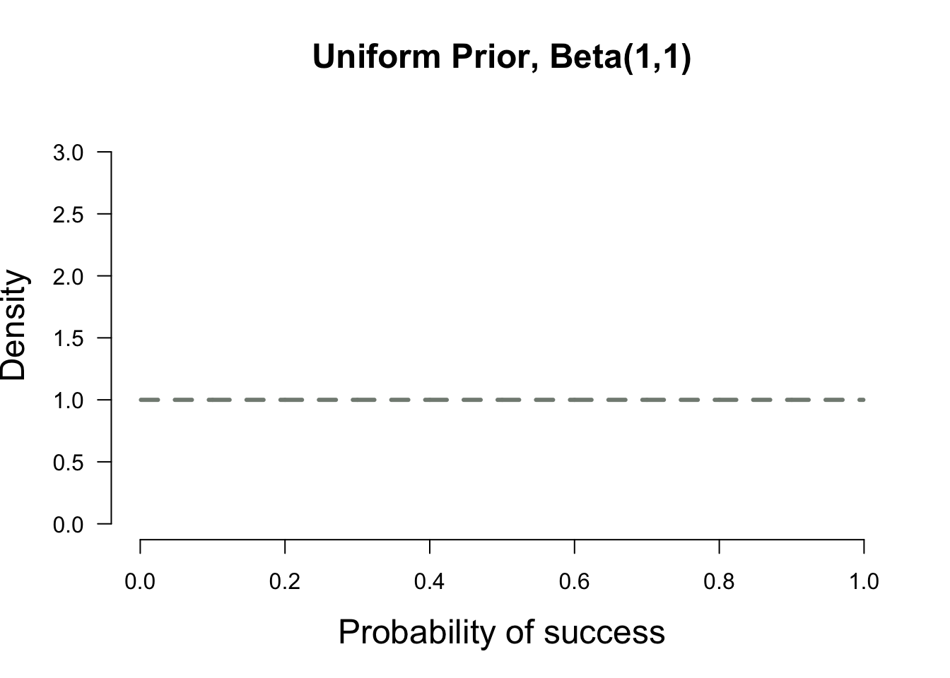
Wanting to gain a little more information you roll over, grab your phone and search Google. You find an article that says that only 12% of the population will get the flu in a given year. But another article says that the prevalence could be a little higher. In this case a distribution of our prior belief might be more appropriate to incorporate our uncertainity. This distribution is known as the prior distribution. In particular, this is called an informed prior distribution because you are incorporating your previous beliefs in the model
plot.beta(12,88,ymax=15,main="Informed Prior, Beta(12, 88)")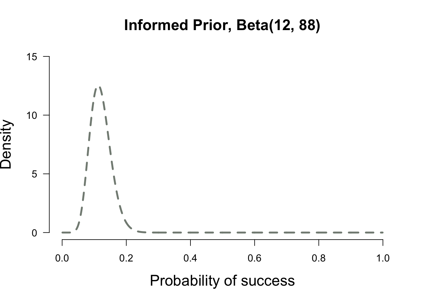
✏ In Bayesian inference, the beta distribution is the conjugate prior probability distribution for the binomial distribution. Computing a posterior using a conjugate prior is very convenient, because you can avoid expensive numerical computation. You can learn more about conjugate priors here
likelihood
The second ingredient is likelihood, this is where we extract information from our data. Likelihood function is the workhorse of bayesian inference. This also appears prominently in frequentist methods. It is very important to understand likelihood for making inferences so it is worth going into a little more detail than what will be covered here. This blogpost is an excellent starting point
Lets say you go out and collect data from 100 of your colleagues and 30 of them also have headache or sore throat but they don’t have a diagnosis. The likelihood curve wil look like this:
x = seq(.001, .999, .001) ##Set up for creating the distributions
y2 = dbeta(x, 1 + 30, 1 + 70) # data for likelihood curve, plotted as the posterior from a beta(1,1)

plot(x, y2, xlim=c(0,1), ylim=c(0, 1.25 * max(y2,1.6)), type = "l", ylab= "Density", lty = 3,
     xlab= "Probability of success", las=1, main="Likelihood Curve for Symptoms Data",lwd=2,
     cex.lab=1.5, cex.main=1.5, col = "cyan3", axes=FALSE)
axis(1, at = seq(0,1,.2)) #adds custom x axis
axis(2, las=1) # custom y axis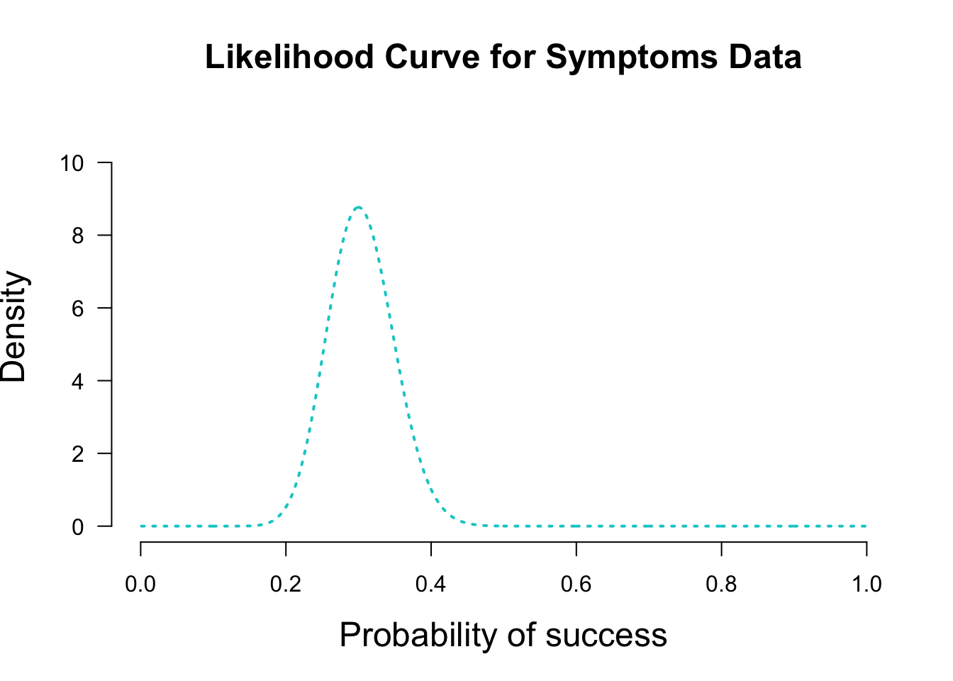
The Likelihood Principle states that the likelihood function contains all of the information relevant to the evaluation of statistical evidence. In other words, facets of the data that do not factor into the likelihood function are irrelevant to the evaluation of the strength of the statistical evidence. The likelihood function is the most compact summary of the data that does not loose information.
is likelihood a probability?
Likelihood is not a probability, but it’s proportional to it.
The likelihood of a hypothesis (\(\theta\)) given some data (Data) is proportional to the probability of obtaining D given that H is true, multiplied by an arbitrary positive constant (K).
Since a likelihood isn’t actually a probability it doesn’t obey various rules of probability. For example, likelihood need not sum to 1.
A critical difference between probability and likelihood is in the interpretation of what is fixed and what can vary. The distinction is subtle, so pay close attention. For the conditional probability, the hypotheses is fixed and the data vary. For likelihood, the data are a given and the hypotheses vary.
posterior
Now for the easiest part. Getting the posterior distribution. This is the distribution representing our belief about the parameter values after we have calculated everything on the right hand side taking the observed data into account.
\(Posterior \propto Prior * Likelihood\)
wait, why did we ignore the demonimator?
Sometimes also called as the evidence, P(data) is simply just a constant, particularly it is a normalizing constant. You’ve already observed the data so you can calculate P(data). One of the necessary conditions for a probability distribution is that the sum of all possible outcomes of an event is equal to 1. The normalising constant makes sure that the resulting posterior distribution is a true probability distribution by ensuring that the sum or integral of the distribution is equal to 1.
Coming back to our example, so far we have two distributions: prior and likelihood. We can get the posterior by multiplying the two. The resulting distribution is shown below
plot.beta(1,1,31,71,ymax=10,main="Beta(1,1) to Beta(31,71)")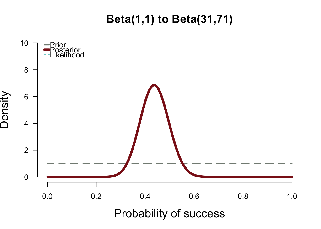
With the uniform prior, the posterior falls right on top of the likelihood function. In the plot above, the likelihood is nearly invisible because the posterior sits right on top of it. When the prior has only 1 or 2 data points worth of information, it has essentially no impact on the posterior shape
plot.beta(12,88,42,158,ymax=15,main="Beta(12,88) to Beta(42,158)")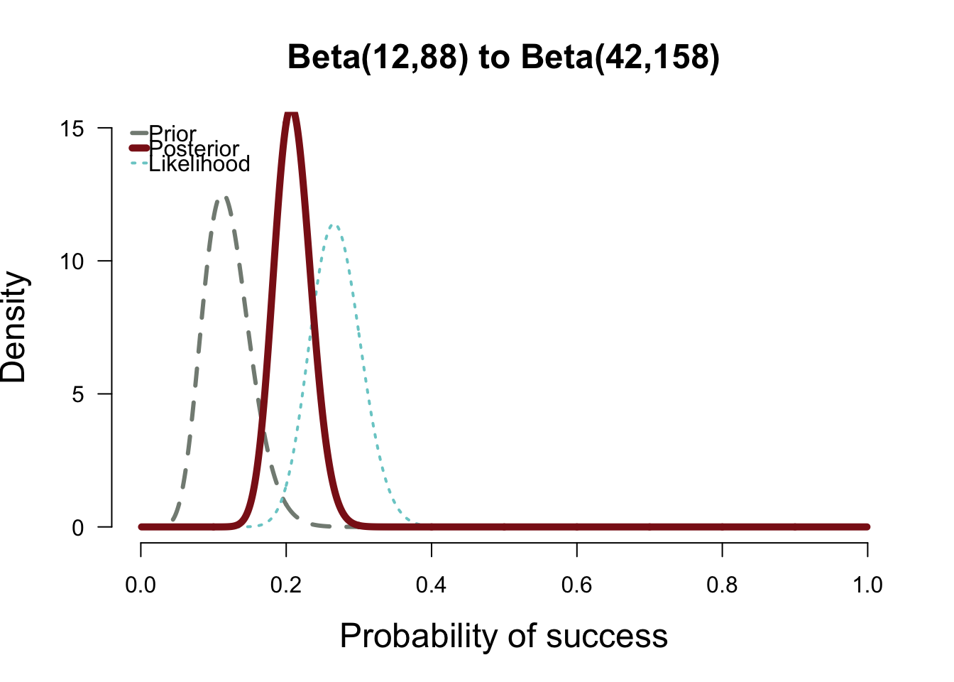
The second plot above shows how the posterior splits the difference between the likelihood and the informed prior. My takeaway is that the the probability of having the flu based on the data you’ve collected is about 20% which is slightly higher than the prior.
Now we have the posterior distribution, we can derive statistics from it. For example, we could use the expected value of the distribution. Or we could calculate the variance to quantify our uncertainty about our conclusion. One of the most common statistics calculated from the posterior distribution is the mode. This is often used as the estimate of the true value for the parameter of interest and is known as the Maximum a posteriori probability estimate or simply, the MAP estimate. But that’s for another time
final thoughts
While there are several advantages of bayesian analysis, it is not without objections. Andrew Gelman discusses some of them in this excellent paper. My personal take is that it in the best interest of the statistician to be knowledgable in both these methods to be able to see through critiques and defences of both these methods