Hello and welcome to my brand new website! I’ve started this blog to think through various statistical concepts and techniques and hopefully they’ll be useful to you too. Let’s start with every statisticians favorite flex: hypothesis testing
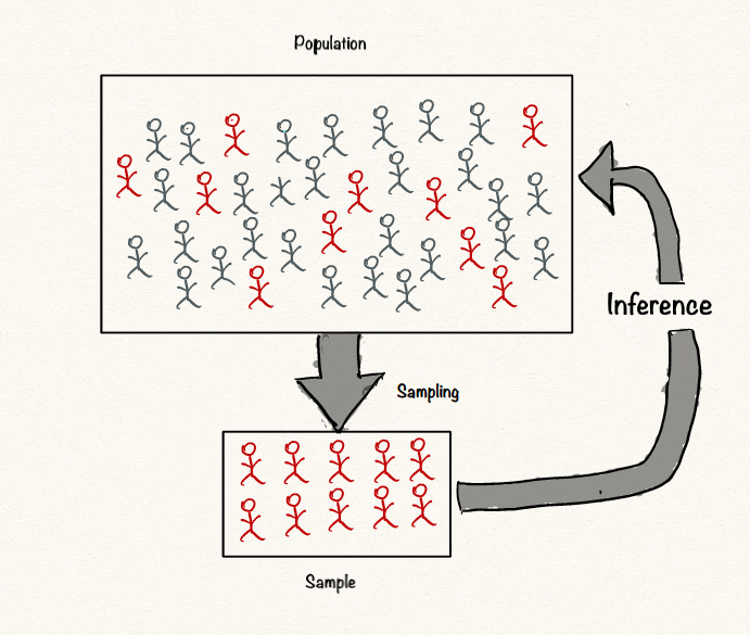
There’s two main branches of statistics. One, where we analyze and summarize the data we have. Other where we infer stuff about a population based on some sample data we collect. This is called inferential statistics and hypothesis testing is an important part of it. It can be confusing because there are endless terminilogies and rules to keep in mind but we can tackle it by breaking it down into smaller parts.
It starts with a hypothesis.
A hypothesis is simply just a question about something in the world around you that can be tested, either by experiment or observation. For example, you may be interested in knowing
Let’s say you’re interested in finding out if coffee stunts your growth. Instead of collecting real data, we just simulate data for adolescent coffee drinkers, assuming a real effect of Cohen’s \(\ d = 7/15\)
set.seed(666)

x <- rep(0:1, each = 50)
y1 <- rnorm(50, mean = 175, sd = 15)
y2 <- rnorm(50, mean = 170, sd = 15)
dat <- data.frame(y = c(y1, y2), x = x)

boxplot(y ~ x, dat, col = c('red', 'grey'),
        xlab = 'coffee drinking status', ylab = 'height')
It seems like the the sample mean height of people that drink coffee is lower than those who don’t. Does that conclude our study? Should we call it a day?
Let’s take a step back for a moment and restate why we should use a hypothesis test rather than just use the sample means to decide. Samples are a subset of the entire population. Sample statistics, such as the mean, are unlikely to equal the actual population values. The difference between the sample value and the population value is called sample error. If sample error causes the observed difference, the next time someone performs the same experiment the results might be different. Hypothesis testing incorporates estimates of the sampling error to help you make the correct decision.
Now that it’s clear why we should be doing hypothesis testing. Below is a rough template to carry out hypothesis testing.
A population parameter of interest is the value(usually mean) we’re hypothesizing on with our data. In our case, the population parameter of interest is
\(\mu\) = mean height for coffee drinkers
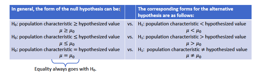
In general terms the hypothesis can be:
The null hypothesis, denoted by \(H_0\), is a claim about a population characteristic that we initially assumed to be true.
The alternative hypothesis, denoted by \(H_1\), is the competing claim (we often set up hypotheses in hopes of showing that \(H_1\) is true).
In carrying out a hypothesis test of \(H_0\) versus \(H_1\), the hypothesis \(H_0\) is rejected in favor of \(H_1\) only if sample evidence strongly suggests that \(H_0\) is false. If the sample does not provide such evidence, then \(H_0\) is not rejected.
Therefore the two possible outcomes of a hypothesis test are reject \(H_0\) or fail to reject \(H_0\) (in some cases we say “fail to reject \(H_0\) in favor of \(H_1\)”).
:exclamation: :exclamation: failing to reject H0 does not mean that we accept H0. :exclamation: :exclamation:
:pencil: Many people have found an analogy between hypothesis testig and court room to be useful where
Below is the general form in which you can set up your hypothesis
In the context of our example,
\(H_0\): \(\mu_c\) = \(\mu_{nc}\)
\(H_1\) = \(\mu_c\) \(\neq\) \(\mu_{nc}\)
where \(\mu_c\) = mean height of the coffee drinking population and \(\mu_nc\) = mean height of the population that doesn’t drink coffee
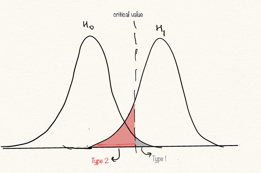
Once hypotheses have been formulated, we need a method for using sample data to determine whether \(H_0\) should be rejected or not. The method that we use is called a test procedure. Unfortunately, just as a jury may reach the wrong verdict in a trial, there is some chance that the use of a test procedure based on sample data may lead us to the wrong conclusion about a population characteristic.
Type 1 error = \(P(reject \ H_0 / H_0 is true)\)
Type 2 error = \(P(fail to reject H_0 / H_1 is true)\)
In keeping with the jury example,
Type 1 error ==> say guilty, when in fact, not guilty
Type 2 error ==> say not guilty, when in fact, guilty
:heavy_exclamation_mark: :heavy_exclamation_mark: Neglecting to think adequately about possible consequences of Type I and Type II errors can lead to severe consequence. this trade off should be made based on the context of the problem :heavy_exclamation_mark: :heavy_exclamation_mark:
but what does setting a significance level mean?
It represents our tolerance for type 1 error. It’s usually repesented by \(\alpha\). Ideally, we want to choose a significance level that minimizes the likelihood of one of these errors.i.e. a very small significance level. Significance levels such as 0.05 and 0.01 are common in most fields.
Now that we know the possible errors that we can make and how we should control them, we need to figure out exactly what it is that we mean by “evidence against \(H_0\)”.
Evidence against the null hypothesis comes in the form of a test statistic, TS. A test statistic is a summary statistic that is a function of the sample data on which the conclusion to reject or fail to reject H0 is based. The most common types of test statistics are Z and t test statistic. Here is a link to a comprehensive list
Another important part of any hypothesis test is the decision rule. The decision rule is a procedure that tells us when to reject or not to reject H0 and is based on the test statistic. Statisticians describe these decision rules in two ways - with reference to a P-value or with reference to a region of acceptance
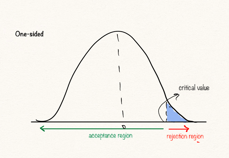
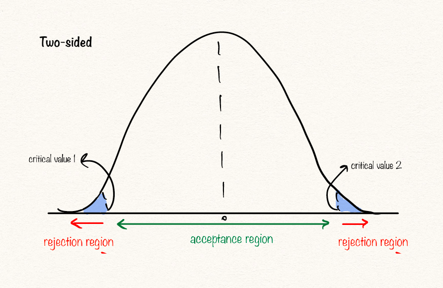
The range of values over which we do not reject H0 is called the acceptance region. The range of values over which we reject H0 is called the rejection region. The number that divides the acceptance and rejection regions is called the critical value.
A critical value is a point (or points) on the scale of the test statistic beyond which we reject the null hypothesis, and, is derived from the level of significance α of the test. Critical value can tell us, what is the probability of two sample means belonging to the same distribution. Higher, the critical value means lower the probability of two samples belonging to same distribution. The general critical value for a two-tailed test is 1.96, which is based on the fact that 95% of the area of a normal distribution is within 1.96 standard deviations of the mean.
However, in practice, most statisticians/ researchers make the decision by computing p-values. Keep in mind p-values are widely misconstructed in the literature. Go through this link for common misconceptions and how to avoid them.
Circling back to our example, we take the p-value route to make a decision. Because the t-test is simply a general linear model with one categorical predictor, we can run:
summary(lm(y ~ x, dat))##
## Call:
## lm(formula = y ~ x, data = dat)
##
## Residuals:
## Min 1Q Median 3Q Max
## -43.120 -10.578 0.219 11.295 33.223
##
## Coefficients:
## Estimate Std. Error t value Pr(>|t|)
## (Intercept) 174.028 2.195 79.293 <2e-16 ***
## x -5.056 3.104 -1.629 0.107
## ---
## Signif. codes: 0 '***' 0.001 '**' 0.01 '*' 0.05 '.' 0.1 ' ' 1
##
## Residual standard error: 15.52 on 98 degrees of freedom
## Multiple R-squared: 0.02636, Adjusted R-squared: 0.01643
## F-statistic: 2.653 on 1 and 98 DF, p-value: 0.1065Putting it in an equation, we can say \(y_i = \beta_0 + \beta_1 x_i + \epsilon\)
In the R output, (Intercept) is \(\beta_0\) while x is \(\beta_1\). \(\beta_0\) is the mean of the group in which our categorical predictor is 0, i.e. the group which does not drink coffee. The group that does drink coffee, on the other hand, has a mean decrease in height of ~5 cm. However, since the p-value is 0.107 We would conclude that the probability of observing these data or more extreme data given that there really is no effect is ~10%. Using the conventional cutoff, \(\alpha = 0.05\), we would say that we fail to reject our null hypothesis that there is no difference between the two groups.